
In the world of data analysis, time is of the essence. No one wants to spend a day setting up an environment or installing packages. Observable Notebooks allows you to dive straight into data exploration so you can focus on what truly matters—turning data into actionable knowledge.
Notebooks are interactive, editable documents defined by code. You can combine formatted text (markdown), code (JavaScript, SQL, HTML), and outputs (e.g. customized data tables and visualizations).
This article will explore 5 features in Observable Notebooks that can revolutionize the way you analyze data, making it faster and more intuitive. You will need to create an account at https://observablehq.com/ and begin your first workspace.
The Dataset
Cattle distribution data in a Google sheet. The data has 3 columns, latitude, longitude, area_name.

The Notebook
From the Observable Workspace, create a new Notebook and import the Google sheet.
# On the google sheet, go to "File > Share > Publish on Web"
# Select CSV and copy the generated url.
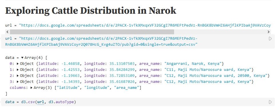
url = "https://docs.google.com/spreadsheets/d/e/2PACX-1vTkXMxqxVF32GCgI7R6MEFtPedVz-RnBGK8bVmHZ6AHjflKPIbaAj9VAVzCoyr2Q078HcG_Kvg4uZTO/pub?gid=0&single=true&output=csv"

# load and parse the CSV file
data = d3.csv(url, d3.autoType)

# `data` is now available for exploration
....
Feature #1: Data Table Cell
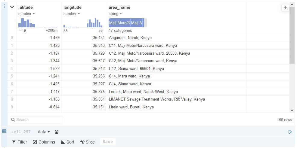
The data is now available for exploration. Begin by quickly browsing via a Data Table Cell. This view presents the data in tabular form. Some of the data wrangling options available are:
- Filter – Limit displayed results to matched criteria.
- Columns (Show/Hide) – Show or hide only certain columns.
- Derive columns – create new columns derived from the original columns using JavaScript.
- Sort – Sort columns into ascending or descending order.
- Slice – Define a slice of data so that only limited rows are shown.
Feature #2: Derived Columns
Since our data points are highly granular, we may want to group relatively close regions for better results. We use a Javascript expression to add a new column named cordinates by concatenating the latitude and longitude column both rounded off to 4 decimal places (0.0001 of a degree is ~11 metres, close enough for our use case).
# [-1.33063598, 35.69580666]  -->   "-1.3306,35.6958"
row["COLUMN"] = row["latitude"].toFixed(4) + "," + row["longitude"].toFixed(4)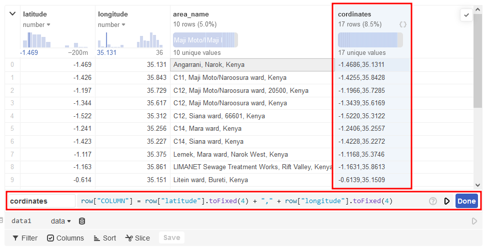
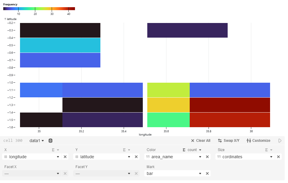
Feature #3: Charts
We can visualize the distribution of the cattle on a chart complete with customization tools.
Feature #4: Interactive Map
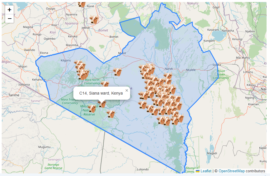
Since our dataset is spatial, we can visualize it on a map using Leaflet. We will represent each location with a custom icon of a cow. We will also draw the Narok boundaries of interest using an Arbitrary Narok GeoJSON file.
narokGeoJson = d3.json("https://res.cloudinary.com/ken-murage-2050/raw/upload/v1723066403/sample_data/jclhk74m7mqb969u1u6x.json")Leaflet Code
map = {
    const container = yield htl.html`<div style="height: 600px;">`;
    const mapCentre = [-1.284043, 35.54945]
    const map = L.map(container).setView(mapCentre, 9);
    L.tileLayer("https://{s}.tile.openstreetmap.org/{z}/{x}/{y}.png", {
        attribution: "© <a href=https://www.openstreetmap.org/copyright>OpenStreetMap</a> contributors"
    }).addTo(map);

    // Custom cow icon
    const cattleIcon = L.icon({
        iconUrl: 'https://www.iconarchive.com/download/i2178/aha-soft/agriculture/cow-head.48.png',
        iconSize: [32, 32]
    });

    // Add cattle positions to the map
    for (let i = 0; i < data.length; i++) {
        const row = data[i]
        L.marker([row.latitude, row.longitude], {
                icon: cattleIcon
            })
            .addTo(map)
            .bindPopup(row.area_name)
            .openPopup();
    }

    // Draw Narok County Area of Intrest / Boundaries
    L.geoJSON(narokGeoJson).addTo(map);
}
Results
Feature #5: Form Controls
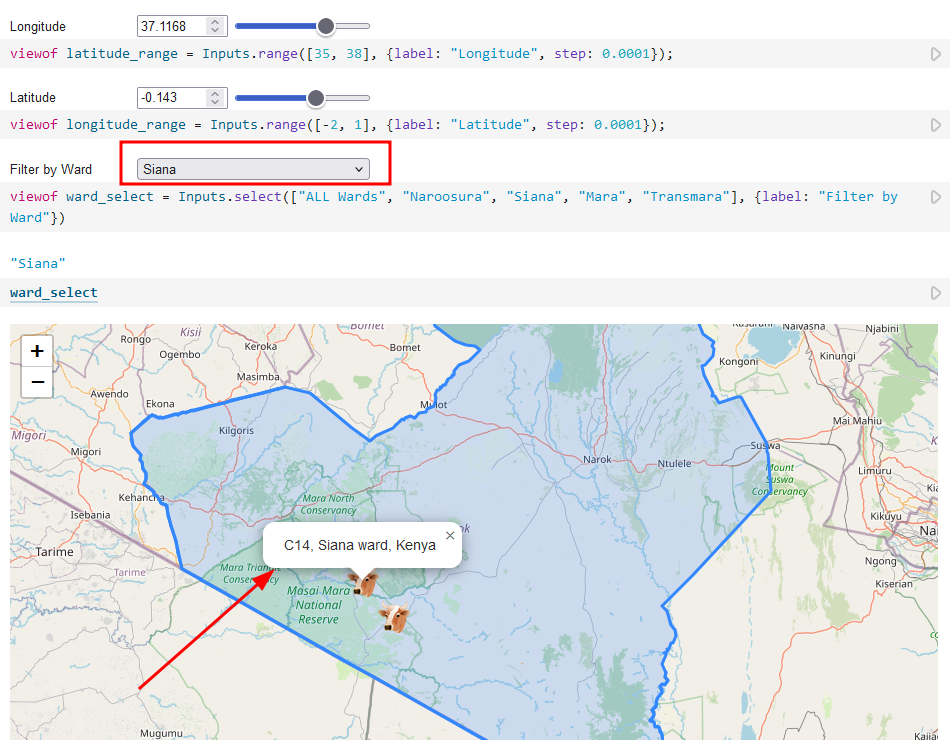
We can also add form controls such as sliders, radio buttons, select boxes etc. For example, if we would like to filter the map by ward names, all we need to add is a select box with the options.
viewof ward_select = Inputs.select(
    ["ALL Wards", "Naroosura", "Siana", "Mara", "Transmara"], {
        label: "Filter by Ward"
    }
)

// Same for Sliders
viewof latitude_range = Inputs.range([35, 38], {label: "Longitude", step: 0.0001});
viewof longitude_range = Inputs.range([-2, 1], {label: "Latitude", step: 0.0001});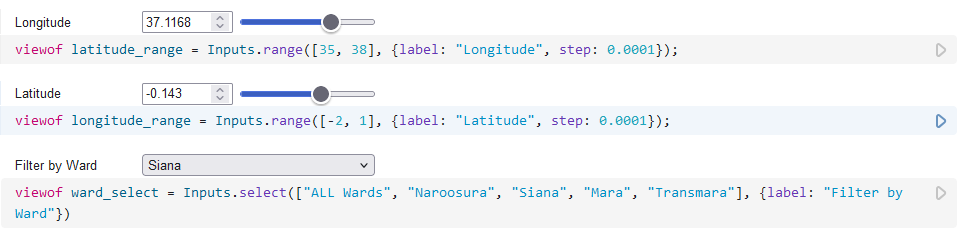
From here we can update the function that adds markers to match points by ward name when adding markers to the map.
// Add cattle positions to the map
for (let i = 0; i < data.length; i++) {
    const row = data[i]

    // if not ALL wards, match the selected item
    if (!ward_select.includes("ALL") && !row.area_name.includes(ward_select)) {
        continue;
    }
    L.marker([row.latitude, row.longitude], {
            icon: cattleIcon
        })
        .addTo(map)
        .bindPopup(row.area_name)
        .openPopup();
}
Results
Conclusion
- Observable notebooks are easy to use, making them accessible to users of all skill levels from beginners to experienced developers. They also integrate with popular viz tools like D3.js and other libraries. Changes to the data are immediately reflected in the notebook e.g. the map above refreshes automatically whenever any of the referenced variables change.
- However, despite the user-friendly interface, there is still a learning curve. Performance for very large datasets or highly complex visualizations can be slow. Observable notebooks run in the browser, which may not handle intensive computations efficiently. They are also cloud-based, meaning you need a stable internet connection to work, offline mode is limited. Not to mention privacy and security concerns with data on the cloud. Finally, advanced features are in the paid-plan.
You may find the complete notebook used in the article here.
Read more on the most popular visualizations at https://observablehq.com/top